DNA modeling

This section specifically focuses on the creation of a DNA molecule and on the way to get it structurally correct

DNA basic 3D modeling
The cubic Bezier tools
Modifying an existing model
Connecting two nucleosomes together
Extending and cyclizing an experimentally-determined DNA structure
How to import a DNA model resulting from simulation?
Connecting modeled DNA to experimental DNA
An example of application: Modeling DNA in a cryoEM map

DNA basic 3D modeling

This video tutorial shows how to create and deform B-DNA

GraphiteLifeExplorer proposes two ways to create DNA: the quadratic Bezier tool (described in this video) and the cubic Bezier tool described in this tutorial.

How to choose between both?

If you want to create a straight DNA molecule, eventually slightly curved, you can use the quadratic tool. The quadratic tool can be used also to create DNA with sharp kink like in the MutS-DNA complex (PDB 1W7A) or the Sac7d-DNA complex (PDB 1AZP).

If the shape you want to create is complicated, prefer the cubic Bezier approach that allows to draw the shape with a few control points. At first glance, the quadratic tool is more intuitive and easier to use. The cubic tool is a little bit confusing the first time but so powerful after 2 or 3 tests!

The cubic Bezier tools

The cubic Bezier tool is useful to create a complicated curved shape with a short number of control points.

GraphiteLifeExplorer proposes two ways to create DNA: the quadratic Bezier tool (described in this tutorial) and the cubic Bezier tool described hereafter.

How to choose between both?

The cubic Bezier tool

0/ A 3D structure (protein or DNA) must be loaded before any DNA modeling task: the reason is that the width of the 3D scene, when empty, is 1 A. This dimension is inferior to the size of one single nucleotide: therefore, the line you draw in the empty space is always less than 1 A, and no base is displayed (remind that the DNA can be described at the atomic level in GraphiteLifeExplorer but a minimum of two nucleotides is displayed).

1/ Go to File, load and choose a PDB file.

2/ Go to Scene, Create Object, choose Line (HexGrid by default) and name the object DNA, press OK. DNA appears in the outliner.

3/ The DNA molecule is not created yet. Go to the “tool” tab, click on the “Create quadratic Bezier curves” button, and add two (control) points in the 3D scene with the Left Mouse Button. Very important: To add a point, it is not enough to click somewhere in the scene, you must drag the mouse (exactly as if you were drawing not a point but a line; in fact, you are drawing a tangent):

4/ You can delete the first structure loaded (here a protein): select the object in the outliner et press on the trash button just above the outliner.

5/ At this stage, before doing anything, check first the mode you are in: in the lower left corner of the screen in the image above, an icon indicates that you are in a “creation” or “modeling” mode (more exactly, in the cubic Bezier mode). Here is a common mistake: you want to turn around an object in the scene (requiring to be in the camera mode) but you add a control point. To delete the newly created point (there is no “undo”): 1/ first transform the point into a tangent. To do so, click on “Edit cubic Bezier curves” (right to the “Create quadratic Bezier curves” button) and drag the mouse from the newly created point: the tangent is created while you drag. 2/ click on the “Create quadratic Bezier curves” button and right-click on the point to delete so that it disappears, and click on the hand-like icon from the “tool” tab or use the Ctrl key to explore the scene.

Note that keeping on pressing the Ctrl key allows to jump to the camera mode (allowing to explore the 3D scene), whatever the current mode is. That’s pretty useful!

6/ Go to the “light” tab and select “curve” instead of “plain”. The DNA axis appears: in fact, one does not draw the DNA from control points but from tangents! Add a third tangent, this will be clearer:

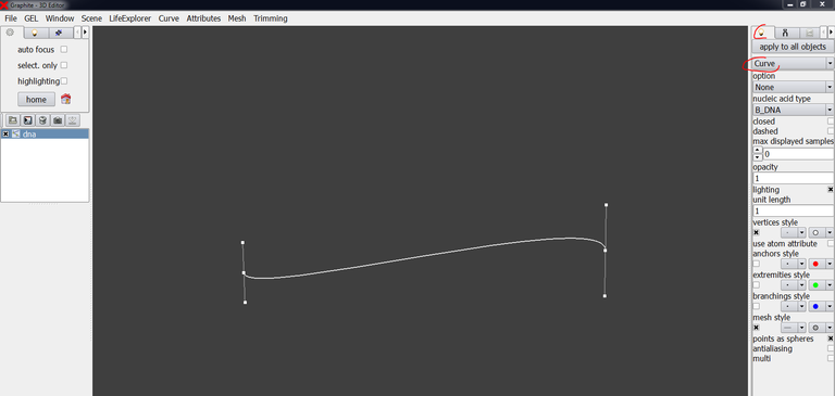
7/ Go to the “light” tab, select “Atoms” instead of “None”, an atomic representation is displayed:

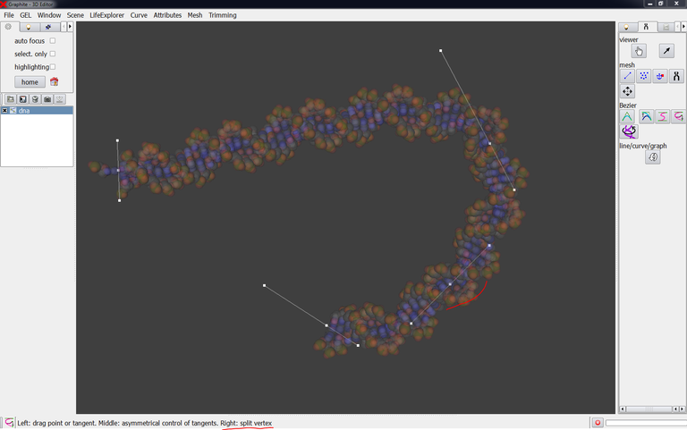
8/ It is obvious that clashes between atoms occur at the apex (red circle on the DNA). We are going to move the middle tangent in order to make the bending less severe. To move and rotate the tangent (by keeping the atomic representation), set “opacity” to 0.2 in the “light tab” so that the points defining a tangent become visible:

In the “tool” tab, click on “Edit cubic Bezier curves”. The icon in the lower left corner indicates the mode you are currently in:

If you move the central point of the tangent (drag with left mouse button), you might not improve the situation. Rather, you’d better move the extreme points to re-orientate the tangent as well as to increase its length. Make some tests and see the behavior of your DNA:

9/ From the image above, the lower left corner indicates what you can do with the tool. In particular, right-click on the last point of the curve and a new tangent is created:

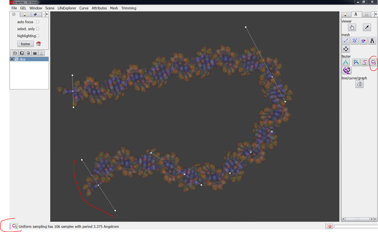
The image below shows the level of complexity a curve can reach thanks to the cubic tool:

This is not a bug:

If you do not drag but you click somewhere in the scene to add a tangent, therefore a point is created and not a tangent:

To get the tangent, click on “Edit cubic Bezier curves” and drag the mouse from the newly created point: the tangent is created while you drag:

Modifying an existing model

This short video tutorial shows how to modify a DNA model

Connecting two nucleosomes together

This tutorial shows how to connect two nucleosomes together for simulation purpose

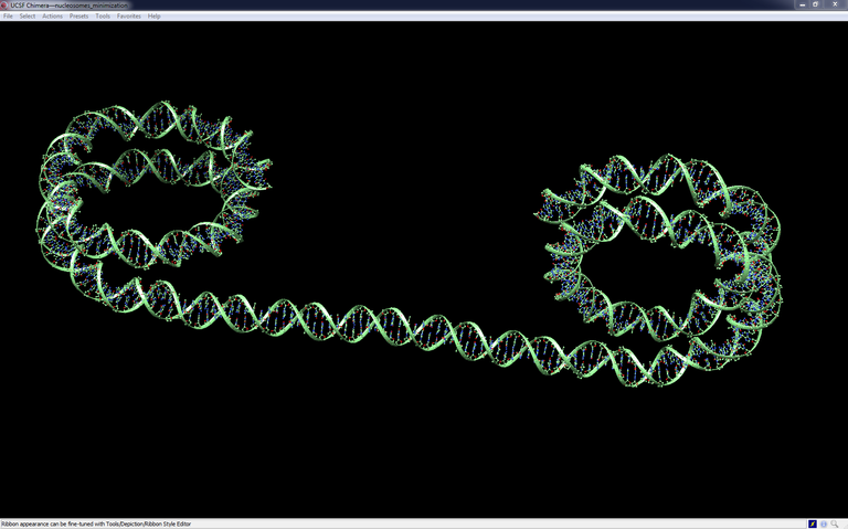
The objective is to create the missing DNA duplex between the two particles and to ensure that the two junctions on both sides are locally structurally correct (as much as possible within the limits of the tools available in the web and of the power of conventional laptops). The model obtained at the end of this detailed tutorial can be a starting configuration for a sophisticated macromolecular simulation able to locate the energetically most stable global conformation of the complex, provide information on the evolution of its conformation in time.

The tutorial is divided this way:

Making the connection
Preparing the minimization
Energetic minimization

Making the connection

1/ Go to the Protein Data Bank and download the nucleosome corresponding to PDB code 1KX5. Remove all HOH atoms recorded as HETATM. Make a copy of the file 1KX5.pdb and name it 1KX5_2.pdb [GraphiteLifeExplorer can not open two instances of a same structure].

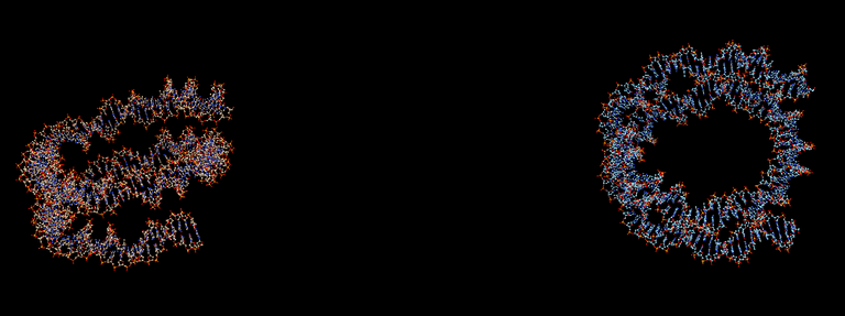
2/ Launch GraphiteLifeExplorer and load PDB 1KX5. Then load 1KX5_2.pdb. Move the structure corresponding to 1KX5_2.pdb to a location in space where you want the structure to stand. This position is an approximation since this second nucleosome will be surely rotated and maybe slightly moved again later:

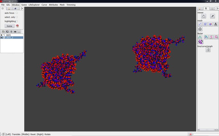
Important notice: Save the scene as decribed here and name it nucleosome.gsg for instance. The folder on your disc contains nucleosomes.gsg plus 1KX5.pdb and 1KX_2.pdb.

We are going to create a DNA duplex and connect it to the first nucleosomal particle:

3/ Display atoms as spheres with point size 2.

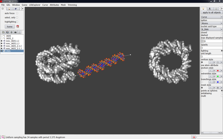
GraphiteLifeExplorer does not make any distinction, visually speaking, between DNA and protein contained in a 3D structure. Therefore you can create a surface for chains I and J corresponding to DNA in order to create the DNA having a connecting role in a more comfortable manner:

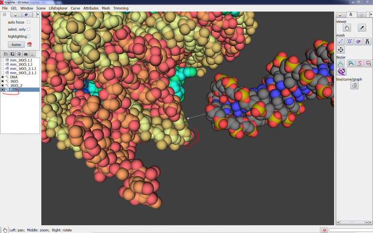
4/ Create (with the cubic Bezier tool) a DNA duplex in the prologation of the nucleosome 1KX5:

At this stage the question is: are the terminal phosphate groups present in the experimental DNA? This knowledge is necessary to model the connecting DNA very accurately: the strands facing each other are polarized the same way and, for a successful energy minimization, the length of P-O3′ bond is less than 3A.

5/ Open 1KX5.pdb and 1KX5_2.pdb in UCSF Chimera (or in your favorite viewer). Choose a standard “ball and stick” representation and delete or hide the aminoacids to show DNA only:

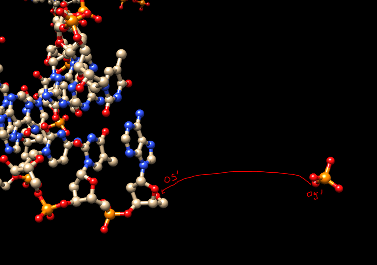
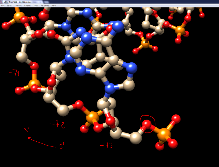
6/ To add missing 5′ phosphates: In Chimera, select a P atom with its 4 oxygen atoms (O3′, O5′, O1P, O2P) from one of the DNA molecule and export them in a single PDB file (from Actions\Write PDB and “Save Selected Atoms only” checked). Name this file P.pdb. Reload this file in your viewer, identify the strand of the first nucleosome where the first residue is -73, and move the newly loaded phosphate group so that the O5′ atom of the phosphate group is superimposed onto the O5′ atom of the first residue:

7/ Still in Chimera save this phosphate group in the PDB file format and

8/ Load it in GraphiteLifeExplorer aand give the atoms of this phosphate group a sphere representation with point size 2:

This phosphate group is going to help us to adjust the connecting DNA to the experimental DNA.

9/ Identify the 3′-end of the connecting DNA. Move the connecting DNA close to the extremity of the experimental DNA by using the translation/rotation tool (curved arrow) available from the Tool tab:

10/ From the Tool tab, click on the Twist tool and select the first base pair (named 0):

11/ Drag with the Right Mouse Button (RMB) to rotate the DNA around its axis and bring its 3′-end in front of the phosphate group recently loaded. To move the camera closer to junction press the Ctrl key while you move the camera with the mouse [once you release the Ctrl key you are instantly back in the previous mode, here the twist mode, as indicated by the the icon in the left lower corner of the screen]:

12/ Adjust the position of the DNA so it looks like in right prologation of the nucleosomal DNA:

13/ You have no way to judge whether the connection is correct or not directly from GraphiteLifeExplorer. Make sure that DNA is selected in the outliner and save it in the PDB file format and name it DNA.pdb.

14/ Open DNA.pdb in a Chimera session already containing 1KX5, display everything as a ball-and-stick representation, and explore the quality of the connection, in particular focuse on the P-O3′ bonds. At this stage, the two P-O3′ length we obtain are 6.242 A and 6.37 A (the connection can be considered as repairable below 3 A):

15/ Go back to GraphiteLifeExplorer and improve the connection. The P-O3′ bond length we obtain here is 2.631 A and 1.831 A:

Let’s consider that the connection with the first nucleosome is satisfying, i.e. the energy minimization process will be able to repair too long bonds. Let’s consider now the connection with the second nucleosome:

16/ Go back to GraphiteLifeExplorer. Modify the position and orientation of the second nucleosome so that one of its DNA “entry” is in the prologation of the connecting DNA. Export 1KX5_2 in the PDB file format [Important notice: name the file 1KX5_3.pdb and rename it 1KX5_2.pdb from its folder. There is a current bug that results in not updating the coordinates if the pdb file carries the same name. It will be fixed].

Notice: When you create a surface (like for the chains I and J of the nucleosomal particles) and then you translate the underlying atomic structure, the surface is not updated (otherwise the user would experience a slowing down of the interactivity). To get the atomic structure and the surface superimposed again, just select the right chain in the GraphiteLifeExplorer window and press “Mesh Surface and Colorize” (exactly as if you wish to create a surface): the surface instantly follows the movement of its underlying atomic structure.

17/ Add a control point to the connecting DNA and adjust its position so that the DNA contacts the DNA of the second nucleosomal particles. Export DNA in the PDB file format (overwrite DNA.pdb):

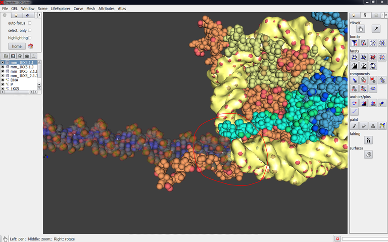
18/ Adjust the position of 1KX5_2 and save it as a PDB file.

19/ Step 19 is entirely carried out in Chimera: Update the Chimera session by loading DNA.pdb and 1KX5_2.pdb. Add a phosphate group (copy P.pdb and name it P2.pdb) to the extremity of the experimental DNA as shown at step 6 and combine this P group to 1KX5_2 by writing a PDB file containing P2.pdb and (1KX5_2.pdbname the file 1KX5_2a.pdb). Then close 1KX5_2.pdb, load 1KX5_2a.pdb, and adjust the position of 1KX5_2a.pdb. Once the connection looks like satisfying (P-O3′ bonds < 3A) overwrite 1KX5_2a.pdb to update the new coordinates.

Preparation for minimization

Our assembly of two nucleosomes connected by a DNA duplex is made of the DNA molecule belonging to the first nucleosome, the DNA molecule belonging to the second nucleosome and the “connecting” DNA. We are going to combine all these DNA molecules in a single PDB file (not to forget the added phosphate groups), rename the chains, renumber the residues, etc.

In Chimera, residue renumbering and chain renaming can be carried out from the menu Tool/Structure Editing.

1/ Let’s start by renumbering residues in chain I of the first nucleosome from 1 instead of -73: the residues are now numbered from 1 to 147.

2/ Chain A of the connecting DNA (DNA.pdb) is in the prologation of chain I of the first nucleosome (1KX5.pdb): rename chain A of DNA.pdb by I and renumber its residues from 148. Chain A ID is now I, and the residues are numbered from 148 to 198 (198 in my model, the value is different in your model).

3/ Chain I of the second nucleosome (1KX5_2a.pdb) is in the prologation of chain I of the connecting DNA, so that no modification of its identifier is required. Renumbered its residues from 199 (instead of -73): the residues are now numbered from 199 to 345 (again, these numbers are different in your situation).

4/ Renumber residues in chain J of the second nucleosome (1KX5_2a.pdb) from 1 instead of -73: the residues are now numbered from 1 to 147.

5/ Chain B of the connecting DNA (DNA.pdb) is in the prologation of chain J of the second nucleosome: rename chain B of DNA.pdb by J and renumber its residues from 148. Chain B id. is now J, and the residues are numbered from 148 to 198 (198 in my model, the value is different in your model).

6/ Chain J of the first nucleosome (1KX5.pdb) is in the prologation of chain J of the connecting DNA, so that no modification of its identifier is required. Renumbered its residues from 199 (instead of -73): the residues are now numbered from 199 to 345 (again, these numbers are different in your situation).

7/ About the P groups: change the ID of the first P group (P.pdb) by J, change its residue number to 199 [type 198 to get 199; I do not know the reason of this behavior in Chimera). change the ID of the second P group (1KX5_2a.pdb, model ID 5.1: remind that P2.pdb and 1KX5_2.pdb were combined at step 19) by I, change its residue number to 199.

8/ Select all the aminoacids and delete them.

9/ Delete the O3′ and O5′ atoms of the P groups and then combine 1KX5.pdb, P.pdb, DNA.pdb, 1KX5_2a.pdb model ID 5.1, and model ID 5.2 into a single PDB file in the reference frame of 1KX5.pdb. Name the PDB file FinalDNA.pdb.

10/ The pdb file thus obtained is to be rearranged in a text editor because it is made of the juxtaposition of 5 models (1KX5.pdb, P.pdb, DNA.pdb 1KX5_2a.pdb model ID 5.1, and model ID 5.2). Do not forget in particular to copy the 3 lines corresponding to one P group and to paste it where they are to be. This is easy to do because the format MODEL ENDMDL allows to find the parts to be reassembled. Also, replace A (for Adenine) by DA, T (fot Thymine) by DT, etc.

Important: Replace C5M by C7

11/ Load FinalDNA.pdb in Chimera and overwrite it again with the Write PDB function in order to renumber the atoms correctly.

Minimization

Notice: This part will be updated as more efficient approaches are brought to our attention and tested. To date structural deficiencies like covalent bond angles greater than standard values resist to the minimization process.

You might not be concerned by this stage as you have home-made minimization algorithms. Hereafter we propose to minimize the structure (FinalDNA.pdb) just obtained. The goal is not to find minimum energy but to clean-up the structure locally as much as possible within the limits of the tools available in the web and of the power of conventional laptops.

Therefore, the user must be aware that this modeling process is to be followed by appropriate molecular dynamics generating rigorous models. One reason is that the connecting duplex must accomodate the mechanical constraint resulting from the attachment to a particle at each of its ends by changing its global shape. The DNA model coming up from the minimization process described below must thus be seen as an intermediate configuration, even if the user considers it to be close to the expected/probable correct geometries taken by the DNA.

1/ Check FinalDNA.pdb with the ADIT validation server and have a look at the validation report. This report indicates structural deficiencies. You can also evaluates clashes with MolProbity.

2/ Go to Tools / Structure Editing and select Minimize Structure.

Keep the default value for Steepest Descent Steps : 100

BUT set Conjugate Gradient Steps to 0 (100 by default)

and press Minimize. Press OK from the successive popup windows (leave the default parameters as such). Chimera looks like stuck with the message Dock Prep finished. Don’t kill Chimera except if nothing happens after 5 or 6 minutes. The minimization starts and ends about 45 minutes later depending on the computer performances.

At the end of the process, save the structure in the PDB format under the name FinalDNA_steepest_minimized.pdb and go back to ADIT. Structural deficiencies like covalent bond angles greater than standard values remain. The use of very recent force field version from AMBER12 is under current testing in Chimera.

Important notice: Set imperatively the Conjugate Gradient Steps to 0 otherwise this particular phase of the minimization process will start after the Steepest Descent has ended. This phase is too long for such a large structure on a common laptop.

Extending and cyclizing an experimentally-determined DNA structure

This tutorial shows how to extend and cyclize a DNA portion contained in an experimentally-determined structure for simulation purpose
The tutorial is useful when one aims at simulating the association of a protein with a DNA duplex thanks to molecular dynamics. The objective of the modeling process detailed here is to provide a structural DNA/protein model (structurally correct at the local scale as much as possible) that can be a starting configuration for a sophisticated macromolecular simulation able to locate the energetically most stable global conformation of the complex, provide information on the evolution of its conformation in time.

The experimental DNA structure 1BNA.pdb is extended from step 1 to 8, cyclized from step 9 to 15, minimized from step 16 to 20.

Applications: If you apply the method with 2AOQ.pdb instead of 1BNA.pdb, therefore you generate a model composed of the protein MutH bound to a DNA duplex. The final model takes into account the local structural effects of MutH onto the DNA. This tutorial can be used to extend DNA in a Holliday junction.

The modeling process is divided this way:

Modeling the extension and making the connections
Preparation to minimization
Minimization

Modeling the extension and making the connections

Here is a snapshot of the GraphiteLifeExplorer interface:

Before using an experimentally solved protein/DNA complex, let’s train ourselves with a “free” experimental DNA (quite less irregular than the structure 2AOQ for instance).

1/ Download PDB 1BNA from the Protein Data Bank, save it on your disk and open it in GraphiteLifeExplorer from the File menu.

2/ Select 1BNA in the outliner, go to the Light tab, select Molecule instead of Plain, and choose “points size” 2.

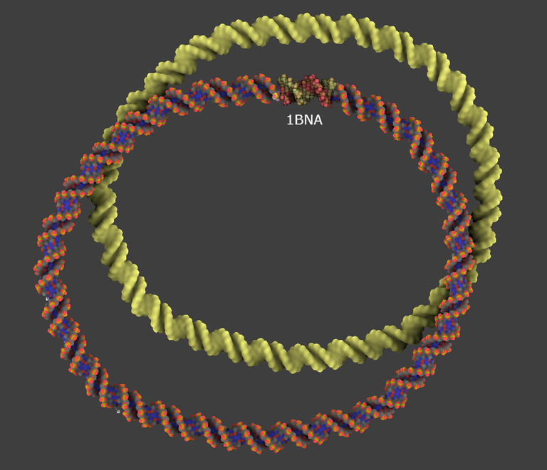
3/ Go to the FX tab and select Ambient occlusion.

4/ Create a DNA model with a circular shape like in the image below and name it mDNA. Use the cubic Bezier tool for that. For your information this is a 270 bp DNA duplex.

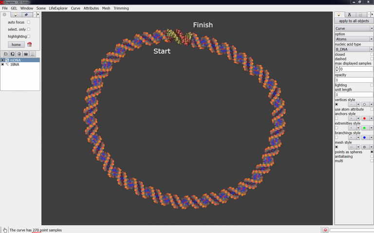
The fine-tuning of the DNA model at each end of the experimentally solved-duplex is the most important step of the whole process. Do not neglect it otherwise the energy minimization will be useless and the structure will be locally not correct.

The difficulty is twofold: 1/ the experimental structure is often uncomplete and atoms useful for modeling can be missing like the 5′ terminal phosphates 2/ the experimental structure is often irregular and there is no reason that the end of the canonical duplex lines up correctly with its target.

Let’s make the first connection.

5/ Use the twist tool to be sure that the strands, when lined up, are polarized the same direction. You can follow steps 6 to 11 here. Another method is to add the missing 5′ terminal phosphates to the experimental structure and to look at this very short tutorial. Adding the missing phosphates will also help to tune the modeled DNA to its target.

To add missing 5′ phosphates: go to your favorite molecular viewer, load 1BNA, select a P atom with its 4 oxygen atoms (O3′, O5′, O1P, O2P) and export them in a single PDB file. Reload this file in your molecular viewer, identify one 5′ end of the nucleic acid structure 1BNA, and move the newly loaded phosphate group so that the O5′ atom of the phosphate group is superimposed onto the first O5′ atom of one the strands. Load another phosphate group and proceed the same way with the other strand:

Obviously, even superimposed onto the O5′ atom, the orientation of a phosphate group is arbitrary. However, once loaded in GraphiteLifeExplorer, it will greatly help to apprehend the distance between the modeled DNA and the experimental duplex. Remind that, if you model the circular DNA so that it remains a distance like 3 Angstroms between the terminal P of the model and the terminal O3′ of the experimental DNA structure, then the minimization aiming at correcting this too long bond will probably fail.

Save the first phosphate group in the PDB file format (in the reference frame of 1BNA) and name it P.pdb. Save the seconde one (P2.pdb).

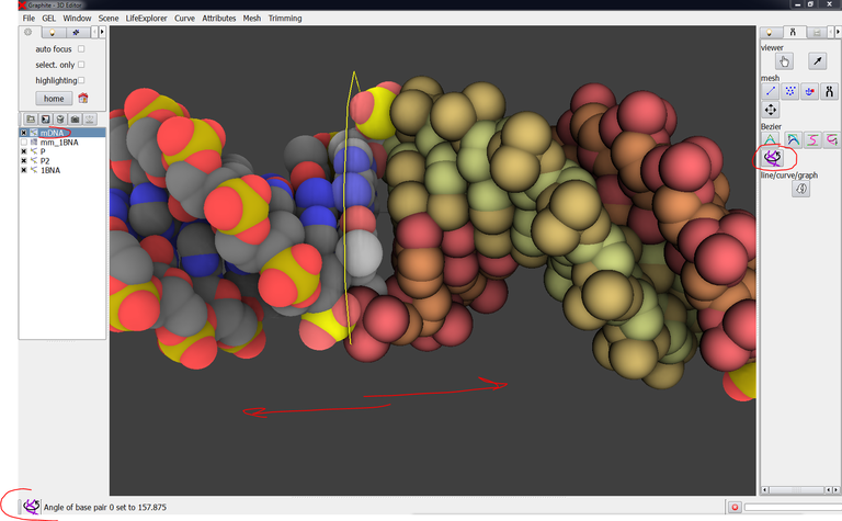
6/ Load P.pdb and P2.pdb in GraphiteLifeExplorer. The image below shows that one 5′-extremity of 1BNA is close to one 5′-extremity of the model DNA: the strands are not correctly polarized:

7/ We must consequently rotate the DNA model around its helical axis. Select mDNA in the outliner, click on the twist tool and select the base pair 0 as shown in the image below. Drag with the right mouse button to rotate the DNA molecule and try to adjust one 5′-end to a 3′-end:

8/ Export the DNA model in the PDB file format and name the file mDNA.pdb. Open this PDB file in UCSF Chimera (or in your favorite molecular viewer) as well as 1BNA.pdb, P.pdb and P2.pdb. The goal is to better know in which extent to adjust the DNA model to 1BNA by using a ball-&-stick representation available in the molecular viewer. Go back to GraphiteLifeExplorer to adjust the DNA model thank to the twist tool. After two or three adjustments, the two P-O3′ bonds connecting the two molecules together are 1.612 A and 1.917 A long, as shown in the image below:

Let’s make the second connection now.

There is no reason that the second extremity of the modeled DNA falls correctly onto the experimental DNA. Getting a correct connection is a matter of DNA length and DNA shape.

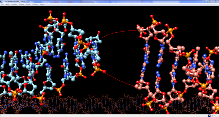
9/ Here is below how the second connection looks like. The two P-O3′ bonds connecting both strands are respectively 10 and 8 A far away. We could use the twist tool to lower the bond length but we would thus take the risk of modifying the structure in an unreasonable manner. We rather recommend to modify the shape and the length to obtain the best possible junction:

10/ From Chimera we notice that the modeled DNA is 2 bp too long. If we reduce the length this way the length of the two P-O3′ bonds remains too long but the P atom and the O3′ atom can be brought closer without rotating the whole structure, just by moving the last control point and fixing the length of the DNA at 268 bp:

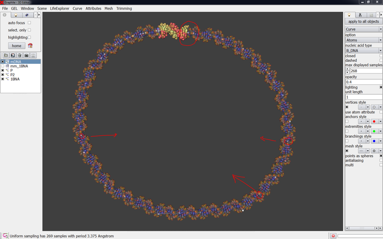
11/ Select mDNA in the outliner and fix the length of the DNA by typing 268 in “max displayed samples”. If you move the last control point you notice that no more base pair is added. Therefore moving the last control point is not the way to bring both DNA molecule close together. Rather changing the global is the way to achieve this.

12/ To bring the DNA molecule closer together we are going to move one or several control points but not the last one. Do the test: Move the third point starting from the last one, you notice that you are able to move the extremity of the modeled DNA [to increase the transparency of the DNA while keeping the atomic representation, turn off ambient occlusion, check lighting, and set opacity to 0.4]:

13/ Try to move some of the control points forming the curve so that the gap between both molecules is reduced:

14/ Export mDNA in the PDB format and load it in Chimera to inspect visually the connection. The connection is not bad: the P-O3′ bond length is respectively 4.577 A and 3.344 A now. But we must do better (the target is < 3 A) by moving one control or more otherwise the energy minimization process will not be able to ensure the structural correctness of the model.

15/ Move some control points and check the result in Chimera. I have been able this way to obtain P-O3′ length of 2.922 A and 2.383 A like in the image below. I stop now the manual modeling to start the minimization process hoping that these bond length (2.922 and 2.383 A) will be lowered.

Export the modeled DNA in the PDB format.

Preparation to minimization

The goal is to combine the modeled DNA, the structure corresponding to 1BNA, the two phosphate groups into a single PDB file.

16/ Load in Chimera the modeled DNA, 1BNA.pdb and the two phosphate groups. Renumber residues, change chain id, to get two chains E and F numbered from 1 to 280. Letters E and F are recommended in order to replace adenine A by DA without any formatting error. Also chain id and numbering of the two phosphate are to be modified and their atoms O3′ and O5′ deleted (they already exist in 1BNA.pdb and in the modeled DNA).

Use the function WritePDB of Chimera to combine all these structures in one single file (in the reference frame of 1BNA.pdb) and name it FinalDNA.pdb.

17/ The pdb file thus obtained is to be rearranged in a text editor because it is made of the juxtaposition of 4 models (corresponding to the modeled DNA, 1BNA.pdb and the two P groups). Do not forget in particular to copy the 3 lines corresponding to one P group and to paste it where they are to be. This is easy to do because the format MODEL ENDMDL allows to find the parts to be reassembled.

Important: Replace C5M by C7

Minimization

18/ Load FinalDNA.pdb in Chimera. The chains are disconnected. Select the P atom and the O3′ atom between residues 1 and 280 in chain E and type the command bond sel to create a bond. Do the same with chain F. The structure is cyclized.

19/ Check FinalDNA.pdb with the ADIT validation server and have a look at the validation report. This report indicates structural deficiencies. You can also evaluates clashes with MolProbity.

20/ Go to Tools / Structure Editing and select Minimize Structure.

Keep the default value for Steepest Descent Steps : 100

BUT set Conjugate Gradient Steps to 0 (100 by default)

and press Minimize. Press OK from the successive popup windows (leave the default parameters as such). Chimera looks like stuck with the message Dock Prep finished. Don’t kill Chimera except if nothing happens after 5 or 6 minutes. The minimization starts and ends about 20 minutes later depending on the computer performances.

At the end of the process, save the minimized structure in the PDB format and go back to ADIT. Structural deficiencies like covalent bond angles greater than standard values remain. The use of very recent force field version from AMBER12 is under current testing in Chimera.

How to import a DNA model resulting from simulation?

GraphiteLifeExplorer is able to rebuild the atomic structure of a simulated double stranded DNA only represented by a curve

(by D. Larivière, Fourmentin-Guilbert Foundation and S. Hornus, INRIA-LORIA)

Tutorial

Note: Graphite-MicroMégas has a new name: Graphite-LifeExplorer. In the screen captures hereafter, read Graphite-LifeExplorer or LifeExplorer instead of MicroMégas

DNA topologies resulting from supercoiling, (dis)entanglement, compaction by proteins, … can be adressed by simulation (see for example http://www.ploscompbiol.org/article/info%3Adoi%2F10.1371%2Fjournal.pcbi.1000678).

A DNA conformation obtained from simulation can be easily exported as a simple curve. MicroMégas rebuilds the atomic structure of the DNA upon this curve. Note that Graphite-LifeExplorer can handle a very long portion of DNA (see explanation at the end).

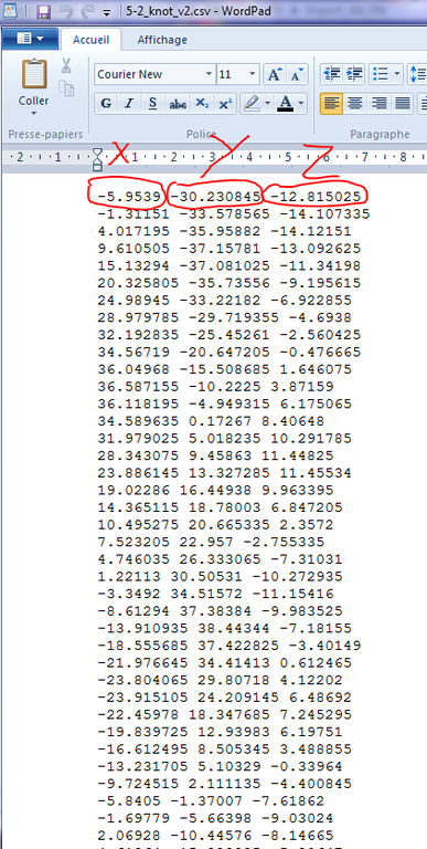
Graphite-LifeExplorer is able to import such a curve, provided the curve is represented by a text file formatted as shown in the image below (3 columns, an empty space between the numbers, a dot instead of a virgule). Each line of the file corresponds to the x,y,z coordinates of a point forming the DNA path:

To import a coordinates file, proceed this way:

1/ Launch Graphite-LifeExplorer

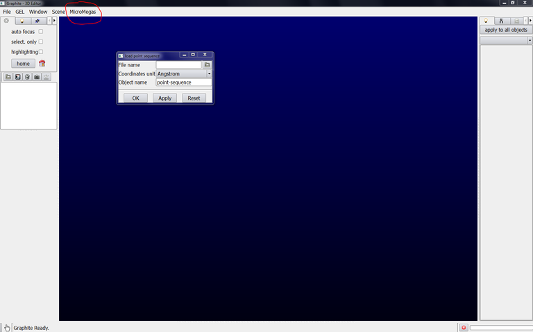
2/ From the main window, go to the Graphite-LifeExplorer menu, select “load point sequence”, a popup window opens:

3/ click on the icon at the right side of File name, select your file (.csv or .dat or.txt like 5-2_knot.csv provided with this tutorial) and press Open:

4/ In the popup window remaining at the screen, select the reference unit of your file: Angstrom or nanometer, rename the object and press OK:

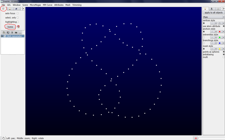
5/ Nothing happens, the scene remains empty.

Go to the tab with an icon representing a wheel gear and click on home, a succession of points (here forming a knot) is displayed:

Important: The choice between Angstom or Nanometer only impacts the length between two points, not the size of the atom nor the diameter of the DNA:

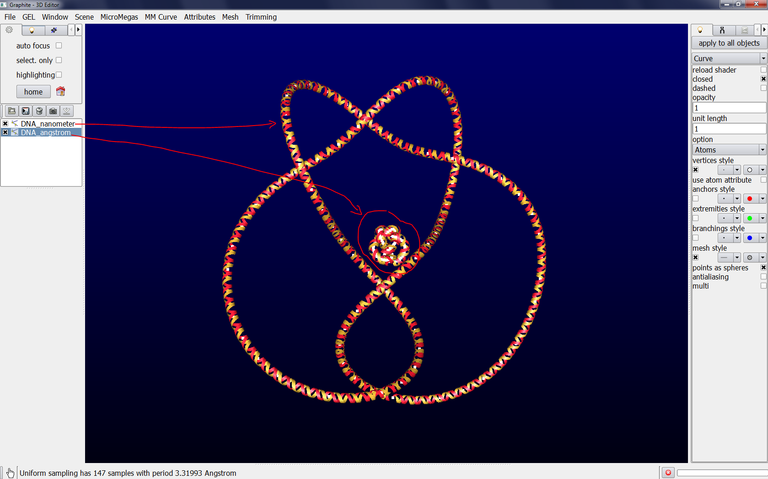
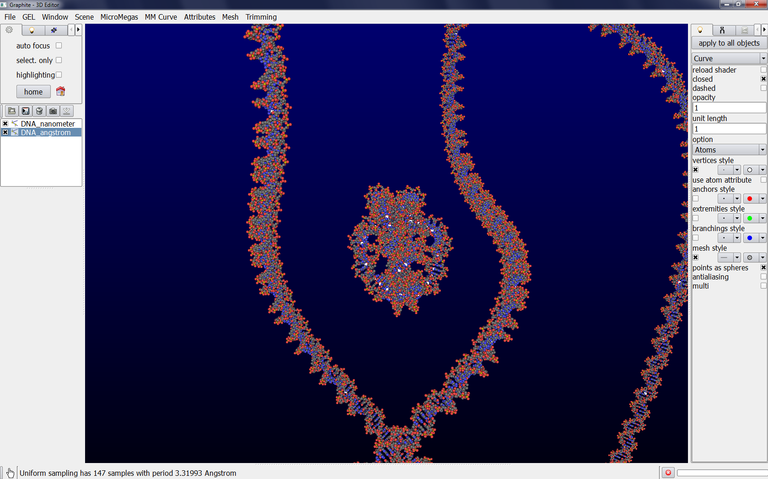
6/ To get an atomic rendering, go to the light tab, select Curve, select Atoms in Option (check closed if you want). A ribbon-like rendering is obtained. When zooming in the scene, the part of the DNA knot closest to the camera is displayed as atoms. This is the level of detail enabling to handle a long portion of DNA without slowing down the machine:

DNA curve

A 5.2 knot (Mathematics of knots is applied to model the action of topoisomerases responsible for keeping DNA unknotted, unlinked, and properly supercoiled)

text/comma-separated-values icon 5-2_knot.csv — text/comma-separated-values, 2 kB (2376 bytes)

Connecting modeled DNA to experimental DNA

This tutorial takes you through the process of connecting a DNA duplex model to a DNA molecule present in an experimental structure.

This tutorial is divided into several parts:

Modeling of the extension (GraphiteLifeExplorer)
Export to the PDB file format and editing (text editor, Chimera)
Making the connection and minimization (HADDOCK)
Back to the modeling session (GraphiteLifeExplorer, Curves+)
Structural validation (ADIT)
Conclusion

At a glance: Extension of the DNA duplex present in PDB 2AOR. This modeling process can be used to create and connect a missing loop at a Holliday junction, or connecting nucleosomes together.

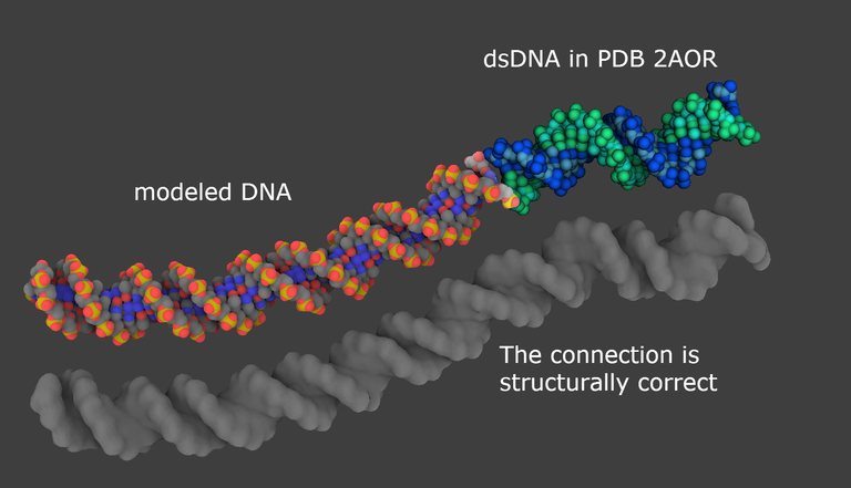
Why such a tutorial? GraphiteLifeExplorer allows the user to draw any arbitrary shape of DNA. However, except for the twist of successive base pairs, the user cannot modify, locally, the atomic structure of a DNA model to render the effects of the interaction with a protein (like inserting the side chain of a protein residue between two base pairs). Yet it is well known that the DNA within a complex often diverges from the canonical curved or straight conformation: Lu and Olson give the examples of the effects on DNA of the Catabolic Activator Protein or the assembly of histone proteins (PMID:18600227). Here we show that GraphiteLifeExplorer can be used together with tools like HADDOCK or Curves+ to extend a duplex present in an experimental 3D structure. The process generates an extended model that includes the structural information present in the experimental structure.

Warning: The user must be aware that this extension modeling process is to be followed by appropriate molecular dynamics generating rigorous models. The reason is that the extended portion must accomodate the mechanical constraint resulting from the connection to a structure at one of its ends or to two structures at each of its ends by changing its global shape. Therefore the DNA model coming up from the process described below must be seen as an intermediate configuration, even if the user considers it to be close to the expected/probable correct geometries taken by the DNA.

Software and web servers: GraphiteLifeExplorer, UCSF Chimera, Haddock, Curves+, ADIT

Required tutorials: The reader should look first at DNA basic 3D modeling and Modifying an existing model.
Modeling the extension (GraphiteLifeExplorer)

1/ Download PDB 2AOR from the Protein Data Bank and save it on your disk

2/ Launch GraphiteLifeExplorer

3/ Go to File and load the file 2AOR.pdb:

4/ Make sure that 2AOR is selected in the outliner, go to the “Light” tab, select the Molecule shader, choose points size 1:

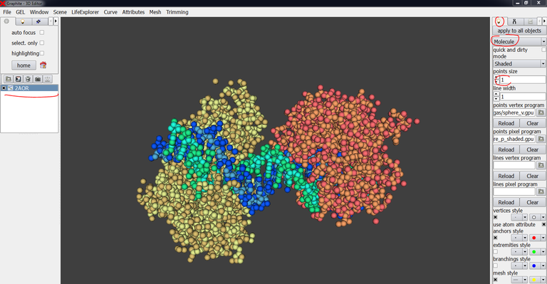
5/ Go to the FX tab and activate ambient occlusion:

6/ DNA is now to be turned to a surface. Go to the GraphiteLifeExplorer window, select Models 1, Chains C, and press Mesh Surface and Colorize:

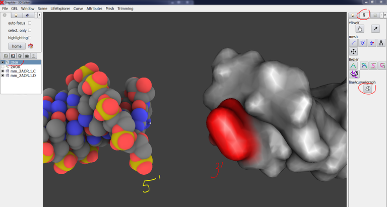
7/ Once the surface has been created, follow exactly the same process for chain D. You obtain the experimental DNA duplex as a grey surface like in this image:

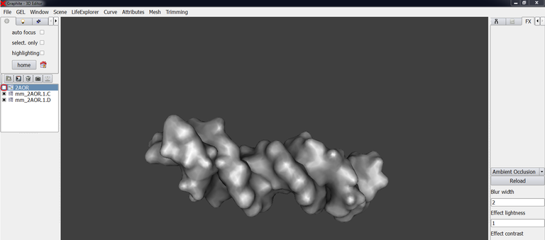
Note: the surface of each strand appears in the outliner and is named mm_2AOR_1_C or D. We can’t create only one surface for the DNA: only separate surfaces for the 4 chains A, B, C and D or a single surface for all chains. To create one single surface for the DNA, one has to edit the PDB file by encapsulating chain C and D with the formalism “MODEL” “ENDMDL”.

Do not forget to save the scene: go to File \ save scene, and give the name connection.gsg (do not format the extension .gsg)

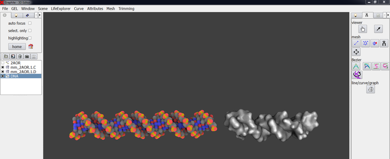
8/ Create a model of straight DNA thanks to the quadratic Bezier curve tool (DNA basic modeling tutorials are required; we do not remind the creation process here). Adjust its position so that it stands correctly in the prologation of the experimental DNA (isosurfaced in grey in the image below):

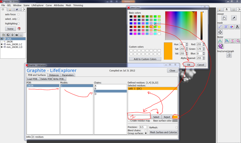
9/ The correct connection of these two structures requires to put face to face strands that are polarized the same way. Regarding the experimental duplex: we use the trick that the residue numbers always increase from 5′ to 3′.

Go to the GraphiteLifeExplorer window, select 2AOR, Models: 1, Chains: C, type 1 in the residue selection box, choose the color orange, press select:

Now, type 22 in the residue selection box, choose the color red, press select, and press Mesh Surface and Colorize:

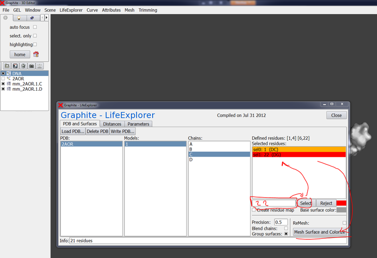
The surface of chain C is now colored in orange at residue 1 (extremity 5′) and in red at residue 22 (extremity 3′):

It is easy to find how a duplex modeled with GraphiteLifeExplorer is polarized (see this tutorial). The strands to be adjusted face to face are recognized:

10/ Zoom on the connection zone (Ctrl key + mouse). We notice that the modeled DNA is to be moved on the right and rotated around its axis:

11/ For that purpose, select DNA in the outliner, click on the move button in the tool tab (arrow-like icon):

… and move DNA to the right with the mouse (left button):

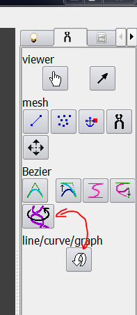
12/ The modeled DNA (named “DNA” in the outliner) is to be rotated around its axis: Select DNA in the outliner, click on the twist tool and select one base pair at the end as shown in the image below:

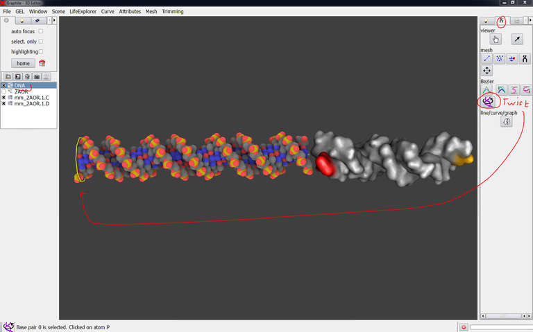
13/ Drag with the right mouse button to rotate DNA around its helical axis:

14/ Click somewhere in the empty space of the 3D view as well as on the Hand icon in order to leave the Twist mode (you should see the message “There is no selected base pair” in the lower corner of the window). The base previously selected in the twist mode remains white colored.

15/ Remind that the Ctrl key allows to use the mouse in the Camera mode. This way the twist tool or another tool can be selected but the Ctrl key activates the camera mode.

16/ Zoom in close to the contact, turn around the contact zone in order to see how far to adjust the modeled DNA to the experimental duplex:

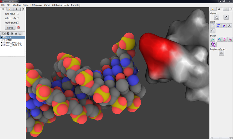
17/ Correctly adjusting both duplexes relative to each other is the difficult step of the whole process. It should be carried out with care since the minimization step will not be able to bring together atoms that are too distant from each other.

Uncheck mm_2AOR.1.C and mm_2AOR.1.D in the outliner, check 2AOR: The structure 2AOR is displayed as a cloud of points. Go to the Light tab, select Molecule, choose points size 2:This ball representation helps to better position the modeled DNA:

18/ However, the part of 2AOR corresponding to the proteins should be hidden. It is not possible to hide a part of a structure in the ball representation. To overcome this limitation, extract the part of the PDB file 2AOR corresponding to the DNA, name it 2AOR_DNA.pdb, and load it in GraphiteLifeExplorer:

19/ Zoom in close to the contact zone. You can check and uncheck mm_2AOR.1.C and mm_2AOR.1.D in the outliner to remember where are the 5′ and 3′ extremities. You notice that one strand seems close enough to the strand to which it is to be paired, while the other one is too far:

20/ When you turn around the objects, you notice that the modeled DNA is to be rotated a bit: to do so, click on the twist tool, select the base previously selected, and drag with the mouse to change the orientation of the DNA. In fact, you alternate between the twist tool (to rotate around the axis) and the translate/rotation tool (to move the object, and rotate it around the center of the scene):

You can obtain this result:

The modeled DNA is now ready to be exported in the PDB file format.

Export to the PDB file format and editing (text editor, Chimera)

The goal of the next few steps is to create a single PDB file containing both the modeled DNA and the experimentally-derived DNA. Chains must be correctly named and residues correctly numbered. This PDB file will then feed the Haddock process of minimization in which missing atoms at the connection will be added and the whole structure refined.

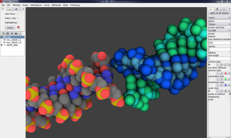
21/ From GraphiteLifeExplorer, export the modeled DNA (named “DNA”in the outliner) in the PDB file format: check “DNA” in the outliner, go to the Curve tab, then Export DNA as PDB, choose a location and name it modeledDNA.pdb. Load the PDB file in a viewer like Chimera as well as the file 2AOR_DNA.pdb. In Chimera, in Actions => Atoms/Bonds => settings, Show backbone as “atoms & bonds, press OK. Again go to the tab Actions, Atoms/bonds, choose balls & sticks: nucleotide objects:

22/ In Chimera, from the menu Tool/Structure Editing, one can change the residue numbering and the chain Id. Do the following modifications:

Chain A of modeledDNA.pdb is turned to E

Chain D of 2AOR_DNA.pdb is turned to E, and the residues are renumbered from 36

Chain B of modeledDNA.pdb is turned to F and residues are renumbered from 23

Chain C of 2AOR_DNA.pdb is turned to F

23/ Go to Actions and select Write PDB. Name the file finalDNA.pdb. In the section « Save models » check the two structures, uncheck « Save selected atoms only », check « Save relative to model : » and choose 2AOR_DNA.pdb, choose « Save multiple models in a single file » and press Save.

24/ Open finalDNA.pdb in a text editor. Delete the formalism MODEL ENDMDL, CONECT. Copy the portion of the file corresponding to “chain E residues 36 to 57” and paste it after the line corresponding to residue 35 of chain E. Copy the portion of the file corresponding to “chain F residues 36 to 57” and paste it after the line corresponding to residue 35 of chain F. Save the file.

The PDB file is not ready yet: the chains are correctly renamed, the residues are correctly numbered but not the atoms:

25/ Open finalDNA.pdb in Chimera, go to Actions and select Write PDB. Name the file finalDNA.pdb. In the section « Save models » check the two structures, uncheck « Save selected atoms only », check « Save relative to model : » and choose 2AOR_DNA.pdb (even if the reference frame now does not matter), choose « Save multiple models in a single file » and press Save.

26/ Open finalDNA.pdb again in a text editor. You notice that atom numbering is correct. Delete the formalism CONECT, add the TER formalism (the TER line for the second chain is not written by Chimera) and save the file.

27/ The last editing step consists of changing the base DA by ADE, DT by THY, DG by GUA, DC by CYT. This is easily done by replacing “DC ” (do not forget the space after DC) by “CYT”. Then, replace A by ADE, T by THY, G by GUA, C by CYT (again, this is easily done by replacing “C ” (do not forget the two spaces after C) by CYT. Note: first change DA, DC, DT, DG and, only then, change A, C, T, G. Add the TER formalism at the end of chains E and F.

And finally, turn residue numbering of chain F from 1 to 58 (all these modifications are mandatory for the HADDOCK process) (note that this renumbering can be done as soon as step 22; we divide the editing process into the maximum possible steps for clarity):

The structure 2AOR.pdb contains non-standard nucleic acids 6MA (N6-Methyl-Deoxy-Adenosine-5′-Monophosphate) that stand as heteroatoms in the PDB file. Replace in finalDNA.pdb “6MA” by “ADE” (which is structurally equivalent) and “HETATM” by “ATOM ” (do not forget the two spaces after ATOM).

The PDB file is ready for being processed in HADDOCK.

Making the connection and minimization (HADDOCK)

The goal of this step is to add missing atoms at the connection and then to minimize the whole structure. Energy minimization aims in particular at correcting the length of O3′-P bonds for instance. Note that this is a minimization carried out at the local scale: do not expect any modification of the whole shape!

The HADDOCK server can not refine only one molecule. We need to create a second molecule that will be refined along with the DNA corresponding to finalDNA.pdb.

28/ From GraphiteLifeExplorer create a very short DNA molecule (3 bp for instance). Take care that 1/ this molecule is not in contact nor superimpose with the DNA previously created and 2/ it is very close to it (we recommend to add this second molecule in the continuation of the DNA to be refined: the reason is that, a bounding box full of water molecule being used during minimization, this way to proceed decreases the number of molecules of water involved in the calculation. Export this molecule in the PDB format and name it secondMolecule.pdb. From Chimera, change chain ids from A to H, and B to I (otherwise the mandatory modifications A to ADE, etc, will pose difficulties). Then, turn A to ADE, T to THY, etc. Delete the CONECT formalism, add the TER formalism. Change residue numbering of chain I from 1 to 5 (chain H stops at residue 4 in my case).

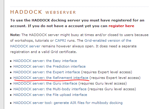
29/ Go to the Haddock web server (you must be registered before using the tool) and select the refinement interface:

29/ Choose finalDNA.pdb as the first molecule. Select “I’m submitting it” and “DNA”. Choose secondMolecule.pdb as the second molecule. Select “I’m submitting it” and “DNA”. Press “Validate” to launch the minimization calculus (it can take hours, depending on the number of queued runs). The server first validates that the PDB files are correctly formatted and then adds the refinement process to the queue.

30/ Once you are informed that your refinement process is successful, download and extract the tar file containing all the solutions and the parameters of your run:

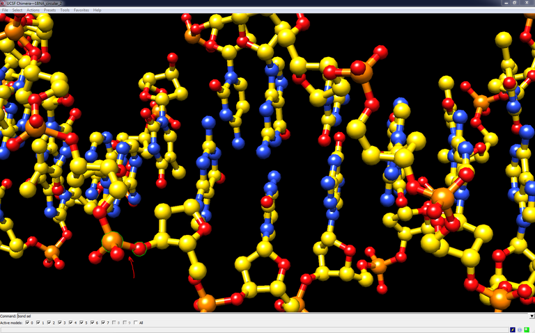
31/ Open the solutions Cluster1_1.pdb, 1_2.pdb, etc in Chimera and look at the connection. In the screenshot below, the “lower” connection is structurally correct while the “upper” one is not: a standard O3′-P bond is not formed, rather a C2′-O5′ is oberved (vertical red arrow). I have to go back to the first step and improve the connection of the modeled DNA to the known DNA. I’m going to move the modeled extension so that the sugar (red circle) comes closer to the phosphate group (blue circle).

Back to the modeling session (GraphiteLifeExplorer, Curves+)

During the first step, we tried to extend the DNA structure contained in 2AOR and made irregular by the interaction with proteins. This is not a trivial task as a canonical DNA molecule (made with GraphiteLifeExplorer) is to be connected to an irregular one.

An information has not been used during the first modeling step: the curvature of the experimentally-derived DNA! The helical axis of 2AOR_DNA.pdb can be viewed in the image below. We notice from the image below that both axis could be better adjusted:

How to get the helical axis of a DNA molecule present in an experimental structure? Not with GraphiteLifeExplorer yet. We can use the Curves+ web server developed by Richard Lavery and coworkers.

32/ Edit in a text editor 2AOR_DNA.pdb in order to replace “HETATM” by “ATOM ” and “6MA” by “DA ” (otherwise Curves+will remove hetero atoms). Both chains in the PDB file are numbered from 1 to 22 in the 5′ – 3′ direction: Renumber (in Chimera) for instance chain D from 23 so that it is numbered from 44 to 23 in the 3′ – 5′ direction.

33/ Go to the Curves+ webserver. Choose 2AOR_DNA.pdb and enter nucleotide numbers like in the image below and press Submit:

34/ A new window opens giving access to the results. Left-click on “PDB helical axis (_X.pdb): data” to download the helical axis under the form of a PDB file:

35/ Go back to GraphiteLifeExplorer and load the structure corresponding to the helical axis, 2AOR_DNA_X.pdb

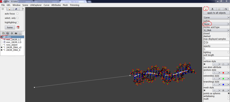
36/ Select 2AOR_DNA_X in the outliner, go to the light tab, select Curve:

37/ Select DNA in the outliner, go to the light tab and choose None instead of Atoms, so that the modeled DNA is displayed as controls points (its helical axis!):

38/ From the image above, we clearly see that the axis of the experimental structure is not prologated by the axis of the modeled extension. You can choose to move the existing modeled DNA and rotate it a little bit. For this tutorial, I prefer starting a new model and use the Cubic Bezier tool that is adequate when one wants to create a curved DNA molecule with a few control points. Delete DNA in the outliner. Create a new DNA model with the Cubic Bezier tool (see this tutorial). Arrange the helical axis so that it looks like in the natural prologation of the experimental DNA axis:

39/ One manner to (eventually) better apprehend the experimental DNA axis in the 3D space is to apply the shader “Molecule”: Select 2AOR_DNA_X in the outliner, go to the Light tab, turn Plain to Molecule and choose “points size 1”:

40/ Use the Twist tool (step 20) to correctly adjust the molecules face to face. Eventually, add supplemental control points close to the junction in order to be able to modify the modeled molecule locally rather than globally. Also, since you have already run a Haddock refinement process, you can replace 2AOR_DNA.pdb in GraphiteLifeExplorer by the part corresponding to 2AOR_DNA.pdb in the HADDOCK solution cluster1_1.pdb in which all atoms are present (thus making the adjustment easier).

41/ Export the model in the PDB format and edit the file (steps 21 to 27).

42/ Refine the model with Haddock (steps 28 to 31).

43/ The HADDOCK solution Cluster1_1.pdb looks like correct in my case:

A priori structurally correct, the whole model is now to be checked with the validation server ADIT of the Protein Data Bank.

Structural validation (ADIT)

44/ HADDOCK is used to renaming all chains of a structure A, B, C,… by a single identifier A (I do not enter in the details but this is relevant for multichain-protein docking). Therefore, since the two complementary strands are named chain A, edit cluster1_1.pdb in a text editor to rename one strand with the identifier B. Add the TER formalism; you can remove the H atoms.

45/ go to ADIT

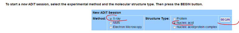
29/ Start the validation process as indicated in the image below:

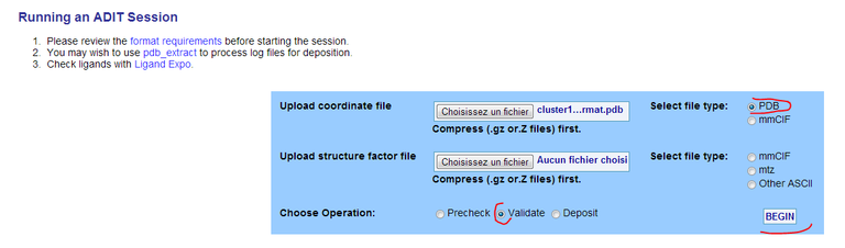
30/ The first output indicates that the coordinate format is OK. Click on “Click here to continue the validation process”.

31/ The second output is the validation report. It mentions bonds and angles that are outside standard values. Everything looks good in our model.

Conclusion

The most important part of the whole process is the GraphiteLifeExplorer modeling task. If it is not carried out carefully, the (local) refinement process with HADDOCK will not be able to connect the experimentally derived DNA molecule and its modeled extension with the right bonds and angles at the junction. Going back to GraphiteLifeExplorer several times in order to improve the extension is expected.

The resulting model is to be seen as an intermediate configuration ready for being processed in simulation experiments.

This modeling process can be used to extend a duplex in an experimental 3D structure, create and connect a missing loop at a Holliday junction, or connecting nucleosomes together. See the tutorials!

An example of application: Modeling DNA in a cryoEM map

In this chapter of Methods in Molecular Biology published with a cryoEM team at IGBMC, we show how GraphiteLifeExplorer can be used to generate a full DNA duplex (155 bp and longer) wrapping around a DNA gyrase pseudo-atomic model that was obtained from cryo-EM data. We show how different DNA lengths can be modeled effortlessly to help design new experiments, formulate hypothesis, or feed Molecular Dynamics simulations.

Olivier Espéli (ed.), The Bacterial Nucleoid: Methods and Protocols, Methods in Molecular Biology, vol. 1624, DOI 10.1007/978-1-4939-7098-8_15, © Springer Science+Business Media LLC 2017

If you do not have access to it, please email us at info@lifeexplorer.eu and we will send you a pdf copy of the protocol.